Training and investigating Residual Nets
The post was co-authored by Sam Gross from Facebook AI Research and Michael Wilber from CornellTech.
In this blog post we implement Deep Residual Networks (ResNets) and investigate ResNets from a model-selection and optimization perspective. We also discuss multi-GPU optimizations and engineering best-practices in training ResNets. We finally compare ResNets to GoogleNet and VGG networks.
We release training code on GitHub, as well as pre-trained models for download with instructions for fine-tuning on your own datasets.
Our released pre-trained models have a higher accuracy than the models in the original paper.
Introduction
At the end of last year, Microsoft Research Asia released a paper titled “Deep Residual Learning for Image Recognition”, authored by Kaiming He, Xiangyu Zhang, Shaoqing Ren and Jian Sun. The paper achieved state-of-the-art results in image classification and detection, winning the ImageNet and COCO competitions.
The central idea of the paper itself is simple and elegant. They take a standard feed-forward ConvNet and add skip connections that bypass (or shortcut) a few convolution layers at a time. Each bypass gives rise to a residual block in which the convolution layers predict a residual that is added to the block’s input tensor.
An example residual block is shown in the figure below.
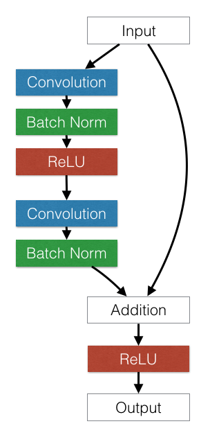
Deep feed-forward conv nets tend to suffer from optimization difficulty. Beyond a certain depth, adding extra layers results in higher training error and higher validation error, even when batch normalization is used. The authors of the ResNet paper argue that this underfitting is unlikely to be caused by vanishing gradients, since this difficulty occurs even with batch normalized networks. The residual network architecture solves this by adding shortcut connections that are summed with the output of the convolution layers.
This post gives some data points for one trying to understand residual nets in more detail from an optimization perspective. It also investigates the contributions of certain design decisions on the effectiveness of the resulting networks.
After the paper was published on Arxiv, both of us who authored this post independently started investigating and reproducing the results of the paper. After learning about each other’s efforts, we decided to collectively write a single post combining our experiences.
Ablation studies (on CIFAR-10)
When trying to understand complex machinery such as residual nets, it can be cumbersome to run exploratory studies on a larger scale – like on the ImageNet dataset – since training a full model takes days to converge. Instead, it’s often helpful to run ablation studies on a smaller dataset to independently measure the impact of each aspect of the model. This way, we can quickly identify the parts of the research that are the most important to focus on during further development. Quick turnaround time and continuous validation are helpful when designing the full system because overlooked details can often bite you in the end.
For these experiments, we replicated Section 4.2 of the residual networks paper using the CIFAR-10 dataset. In this setting, a small residual network with 20 layers takes about 8 hours to converge for 200 epochs on an Amazon EC2 g2.2xlarge instance. A larger 110-layer network takes 24 hours. This is still a long time, but critical bugs that prevent convergence are often immediately apparent because if the code is bug-free the training loss should decrease quickly (within minutes after training starts).
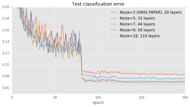
Effects of model depth. The residual networks paper provides a natural starting point for comparison: Figure 6 from the paper simply measures accuracy with respect to the depth of the network. To reproduce this figure, we held the learning rate policy and building block architecture fixed, while varying the number of layers in the network between 20 and 110. Our results come fairly close to those in the paper: accuracy correlates well with model size, but levels off after 40 layers or so.
Residual block architecture.
After validating that our results come fairly close to the original paper, we started considering the impact of slightly different residual block architectures to test the assumptions of the model. For example:
-
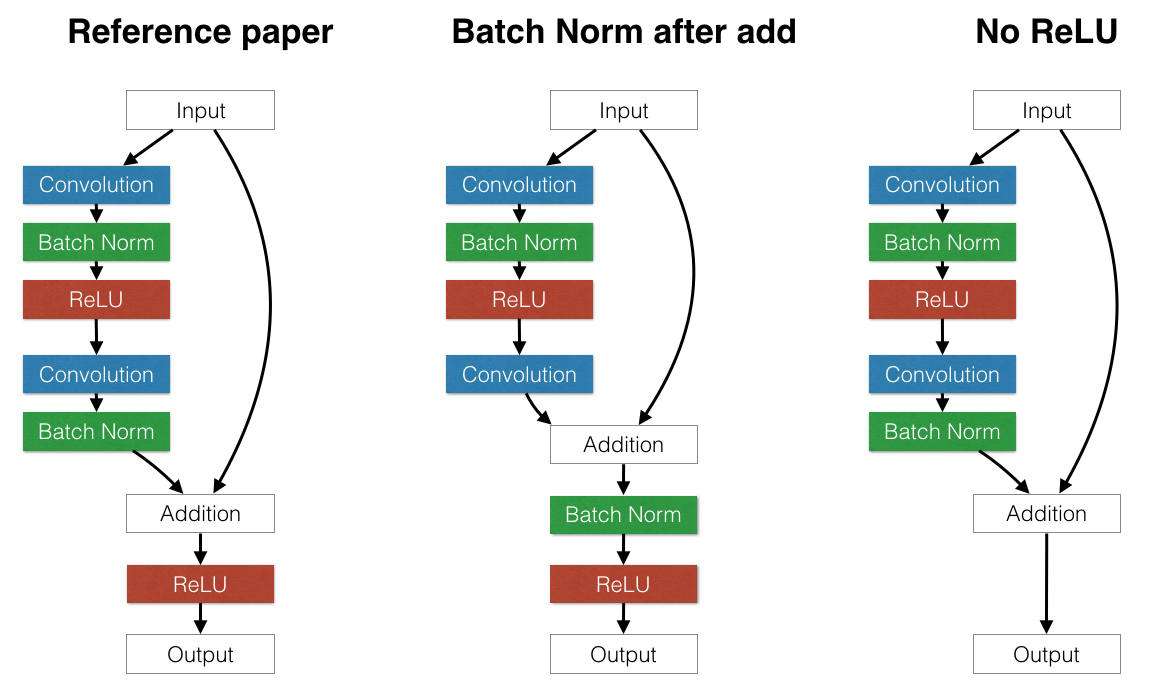
Is it better to put batch normalization after the addition or before the addition at the end of each residual block? If batch normalization is placed after the addition, it has the effect of normalizing the output of the entire block. This could be beneficial. However, this also forces every skip connection to perturb the output. This can be problematic: there are paths that allow data to pass through several successive batch normalization layers without any other processing. Each batch normalization layer applies its own separate distortion which compounds the original input. This has a harmful effect: we found that putting batch normalization after the addition significantly hurts test error on CIFAR, which is in line with the original paper’s recommendations.
-
The above result seems to suggest that it’s important to avoid changing data that passes through identity connections only. We can take this philosophy one step further: should we remove the ReLU layers at the end of each residual block? ReLU layers also perturb data that flows through identity connections, but unlike batch normalization, ReLU’s idempotence means that it doesn’t matter if data passes through one ReLU or thirty ReLUs. When we remove ReLU layers at the end of each building block, we observe a small improvement in test performance compared to the paper’s suggested ReLU placement after the addition. However, the effect is fairly minor. More exploration is needed.
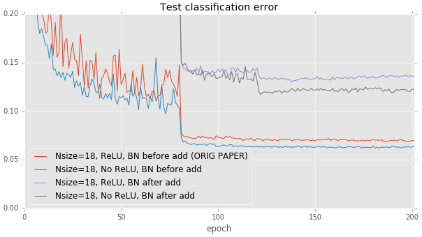
These results were run on the deeper 110-layer models. The effect is much less pronounced on the shallow 20-layer baseline.
Alternate optimizers. When running a hyperparameter search, it can often pay off to try fancier optimization strategies than vanilla SGD with momentum. Fancier optimizers that make nuanced assumptions may improve training times, but they may instead have more difficulty training these very deep models. In our experiments, we compared SGD+momentum (as used in the original paper) with RMSprop, Adadelta, and Adagrad. Many of them appear to converge faster initially (see the training curve below), but ultimately, SGD+momentum has 0.7% lower test error than the second-best strategy.
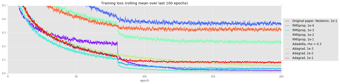
| Solver | Testing error |
|---|---|
| Nsize=18, Original paper: Nesterov, 1e-1 | 0.0697 |
| Nsize=18, Best RMSprop (LR 1e-2) | 0.0768 |
| Nsize=18, Adadelta | 0.0888 |
| Nsize=18, Best Adagrad (LR 1e-1) | 0.1145 |
These experiments help verify the model’s correctness and uncover some interesting directions for future work. However, moving to the much larger ImageNet dataset opens its own Pandora’s box of interesting challenges.
For a more in-depth report of the ablation studies, read here.
Training at a larger scale: ImageNet
We trained variants of the 18, 34, 50, and 101-layer ResNet models on the ImageNet classification dataset.
What’s notable is that we achieved error rates that were better than the published results by using a different data augmentation method.
We are also training a 152-layer ResNet model, but the model has not finished converging at the time of this post.
We used the scale and aspect ratio augmentation described in “Going Deeper with Convolutions” instead of the scale augmentation described in the ResNet paper. With ResNet-34, this improved top-1 validation error by about 1.2% points. We also used the color augmentation described in “Some Improvements on Deep Convolutional Neural Network Based Image Classification,” but found that had a very small effect on ResNet-34.
Model changes
We experimented with moving the batch normalization layer to from after the last convolution in a building block to after the addition. We also experimented with moving the stride-two downsampling in bottleneck architectures (ResNet-50 and ResNet-101) from the first 1x1 convolution to the 3x3 convolution.
| Model | Batch Norm | Stride-two layer | Top-1 single-crop err (%) |
|---|---|---|---|
| ResNet-18 | after conv | 3x3 | 30.6 |
| ResNet-18 | after add | 3x3 | 30.4 |
| ResNet-34 | after conv | 3x3 | 26.9 |
| ResNet-34 | after add | 3x3 | 27.0 |
| ResNet-50 | after conv | 3x3 | 24.5 |
| ResNet-50 | after add | 1x1 | 24.5 |
| ResNet-50 | after add | 3x3 | 24.2 |
Batch normalization
Torch uses an exponential moving average to compute the estimates of mean and variance used in the batch normalization layers for inference. By default, Torch uses a smoothing factor of 0.1 for the moving average. We found that decreasing the smoothing factor to 0.003 and recomputing the mean and variance improved top-1 error rate by about 0.2% points.
Multi-GPU training
Using 4 NVIDIA Kepler GPUs and optimizations described below, training took from 3.5 days for the 18-layer model to 14 days for the 101-layer model.
To speed up training, we used:
Data parallelism over 4 GPUs : This is a standard way of speeding up training deep learning models. The input is a mini-batch of N samples, which are divided into N / 4 sub-batches and sent to each GPU separately for training, and the network parameters are communicated across the GPUs in the process. In torch, this can be done using nn.DataParallelTable.
FFT based convolutions via CuDNN-4 : Using the CuDNN Torch bindings, one can select the fastest convolution kernels by setting cudnn.fastest and cudnn.benchmark to true. This automatically benchmarks each possible algorithm on your GPU and chooses the fastest one. This sped up the time per-mini-batch by about 40% on a single GPU, but slowed down the multi-GPU case due to the additional kernel launch overhead.
Multi-threaded kernel launching : The FFT-based convolutions require multiple smaller kernels that are launched rapidly in succession. Although CUDA kernel launches are asynchronous, they still take some time on the CPU to enqueue. With DataParallelTable, all the kernels for the first GPU are enqueued before kernels any are enqueued on the second, third, and fourth GPUs. To fix this, we introduced a multi-threaded mode for DataParallelTable that uses a thread per GPU to launch kernels concurrently.
NCCL Collectives : We also used the NVIDIA NCCL multi-GPU communication primitives, which sped up training by an additional 4%. 4% might sound insignificant, but for example, when training Resnet-101 this amounts to a saving of 13 hours.
GPU memory optimizations
We used a few tricks to fit the larger ResNet-101 and ResNet-152 models on 4 GPUs, each with 12 GB of memory, while still using batch size 256 (batch-size 128 for ResNet-152). In a backwards pass, the gradInput buffers can be reused once the module’s gradWeight has been computed. In Torch, an easy way to achieve this is to modify modules of the same type to share their underlying storages. We also used the in-place variants of the ReLU and CAddTable modules.
Adding these memory optimizations only amount to an extra 10 lines of code.
Speed of ResNets vs GoogleNet and VGG-A/D
It is interesting to compare ResNets in terms of training / inference time against other state-of-the-art convnet models in the context of image classification. We measured the time for a full forward and backward pass for a mini-batch of 32 images for ResNet, VGG A, VGG D, Batch-Normalized Inception, and Inception v3 on a NVIDIA Titan X. Also listed is the top-1 single-crop validation error on the Imagenet-2012 dataset.
| Model | Top-1 err (%) | Time (ms) |
|---|---|---|
| VGG-A | 29.6 | 372 |
| VGG-D | 26.8 | 687 |
| ResNet-34 | 26.7 | 231 |
| BN-Inception | 25.2 | 192 |
| ResNet-50 | 24.0 | 403 |
| ResNet-101 | 22.4 | 649 |
| Inception-v3 | 21.2 | 494 |
While ResNets have definitely improved over Oxford’s VGG models in terms of efficiency, GoogleNet seems to still be more efficient in terms of the accuracy / ms ratio.
Code Release
We are releasing code for training ResNets so that others can train them on their own datasets. Code for training ResNets on ImageNet is at https://github.com/facebook/fb.resnet.torch. This also includes options for training on CIFAR-10, and we also describe how one can train Resnets on their own datasets.
The code for the CIFAR-10 ablation studes is at https://github.com/gcr/torch-residual-networks.
Pre-trained models
We are releasing the ResNet-18, 34, 50 and 101 models for use by everyone in the community. We are hoping that this will help accelerate research in the community. We will release the 152-layer model when it finishes training.
The pre-trained models are available at this link, and includes instructions for fine-tuning on your own datasets.
Our models have better accuracy than the original ResNet models, most likely because of the aspect ratio augmentation. The table below shows a comparison of single-crop top-1 validation error rates between the original residual networks paper and our released models.
As you see, our ResNet-101 model gets a higher accuracy than MSR-A’s ResNet-152 model. We did not tune our models heavily over the validation error and so haven’t overfitted to the validation set. In fact, we only ever trained one instance of the ResNet-101 model, without any hyperparameter sweeps.
| Model | Original top-1 err (%) | Our top-1 err (%) |
|---|---|---|
| ResNet-50 | 24.7 | 24.0 |
| ResNet-101 | 23.6 | 22.4 |
| ResNet-152 | 23.0 | N/A |
Conclusion
We presented our investigations on model-selection, optimization and our engineering optimizations, in the context of training Deep Residual Nets. We released optimized training code, as well as pre-trained models, in the hope that this benefits the community.
#####################################################################################################################
Acknowledgements
Kaiming He for discussing ambiguous and missing details in the original paper and helping us reproduce the results.
Ross Girshick, Piotr Dollar, Tsung-yi Lin and Adam Lerer for discussions.
Natalia Gimelshein, Nicolas Vasilache, Jeff Johnson for code and discussions around multi-GPU optimization.
References
[1] He, Kaiming, et al. “Deep Residual Learning for Image Recognition.” arXiv preprint arXiv:1512.03385 (2015).
[2] Ioffe, Sergey, and Christian Szegedy. “Batch normalization: Accelerating deep network training by reducing internal covariate shift.” arXiv preprint arXiv:1502.03167 (2015).
[3] Simonyan, Karen, and Andrew Zisserman. “Very deep convolutional networks for large-scale image recognition.” arXiv preprint arXiv:1409.1556 (2014).
comments powered by Disqus