Dueling Deep Q-Networks

April 30, 2016 by Kai Arulkumaran

Deep Q-networks (DQNs) [1] have reignited interest in neural networks for reinforcement learning, proving their abilities on the challenging Arcade Learning Environment (ALE) benchmark [2]. The ALE is a reinforcement learning interface for over 50 video games for the Atari 2600; with a single architecture and choice of hyperparameters the DQN was able to achieve superhuman scores on over half of these games. The original work has now been superseded with several advancements, several of which can be found on GitHub. As training on the ALE can take over a week on a GPU, the code is also set up to learn how to play a simpler game of catch in a couple of hours on a CPU.

Reinforcement Learning

Most recent deep learning research has focused around supervised learning, which involves finding a mapping from input data \(x\) to target data \(y\). Specifically, neural networks are parameterised functions, \(f(x; \theta)\), where we learn the parameters \(\theta\) by using an error signal. Unsupervised learning involves inferring structure about the input data, has no such signal, and can be approached in several ways (for example, clustering). Reinforcement learning instead utilises a reward signal, with no explicit mapping from input to target data, but instead a goal of maximising the reward it receives.

In the reinforcement learning scenario, an agent has to learn by interacting with its environment through trial and error. Formally, we consider the environment with a set of states \(\mathcal{S}\), and the agent having a set of actions \(\mathcal{A}\). At each discrete time step, \(t\), the agent observes the state of the environment \(s_t\) and chooses an action \(a_t\) to perform. The agent then receives a scalar reward \(r_{t+1}\), and observes the next state, \(s_{t+1}\). This action-perception loop is shown in the figure below.

Meanwhile, the agent seeks to learn a (control) policy \(\pi\) which it uses to determine which action to perform given its current state. The best action is the one that maximises its expected return, \(\mathbb{E}[R]\), where \(R\) is defined as follows:

\[R = \sum\limits_{t=0}^{T-1} \gamma^tr_{t+1}\]

In the context of video games, \(R\) is the sum of all the rewards (increments in score) received in one episode (until the player dies) that lasts for \(T\) discrete time steps (which are usually the individual frames). We also use a discount variable, \(\gamma\), which determines how “far-sighted” the agent is - a value of 0 means that the agent only cares about the next reward it receives, whilst a value of 1 means that it cares equally about every reward it will receive in the future.

One technique for solving reinforcement learning problems is Q-learning, which involves learning an action-value function:

If we had the optimal action-value function available to us, then the policy would be as simple as taking the action that maximises the function depending on the state the agent is in, for every single time step. However, the optimal function isn’t available to us, so we have to try and learn it from experience. At every time step, when the agent performs an action, it’ll receive a reward. The goal is to update \(Q\) based on an error, \(\delta\), along with a learning rate, \(\alpha\):

\[Q_{t+1}(s_t, a_t) = Q_t(s_t, a_t) + \alpha \delta\]

\(\delta\) is the difference between the current value of \(Q\) and a target \(Y\), which itself is the reward received plus the discounted max Q-value of the next state:

\[\delta = \left(r_t + \gamma\max_aQ_t(s_{t+1}, a)\right) - Q_t(s_t, a_t)\]

Deep Q-Networks

Coming back to deep learning, it makes sense that rather than learning \(Q\) exactly, we can approximate it with a deep neural network. Indeed, neural networks have been used in the past with great success on reinforcement learning problems [3], even using Q-learning [4]. So for playing Atari 2600 video games, if we want to learn from the raw pixels on the screen - the observed state of the environment - then it makes sense to start with a convolutional neural network (CNN), and this is exactly what the DQN does [1]. We could also feed a neural network a one-hot encoding of the action, and get out the Q value from one unit at the top, but there is a more efficient way to do this. This is the first trick of DQNs - they only take the screen as input, and output the Q value for each possible action at the top. Not only does this reduce computation (as opposed to running the network for each action), but we would expect that the lower convolutional parts of the DQN would not really be affected by the action anyway. This way the lower part focuses on extracting good spatial features, whilst the upper part with fully connected layers can focus more on the consequences of the different actions. The network architecture is then rather straightforward:

local net = nn.Sequential()
net:add(nn.View(histLen * nChannels, height, width)) -- Concatenate frames in channel dimension
net:add(nn.SpatialConvolution(histLen * nChannels, 32, 8, 8, 4, 4, 1, 1))
net:add(nn.ReLU(true))
net:add(nn.SpatialConvolution(32, 64, 4, 4, 2, 2))
net:add(nn.ReLU(true))
net:add(nn.SpatialConvolution(64, 64, 3, 3, 1, 1))
net:add(nn.ReLU(true))
net:add(nn.View(convOutputSize))
net:add(nn.Linear(convOutputSize, hiddenSize))
net:add(nn.ReLU(true))
net:add(nn.Linear(hiddenSize, m)) -- m discrete actions

A significant component of the DQN training algorithm is a mechanism called experience replay [5]. Transitions experienced from interacting with the environment are stored in the experience replay memory. These transitions are then uniformly sampled from to train on in an offline manner. From a theoretical standpoint this breaks the strong temporal correlations that would affect learning online. From a more practical perspective this not only allows data to be reused, but also allows for hardware-efficient minibatches to be used.

Another component of the training algorithm is the target network. Function approximation in reinforcement learning can be unstable, so the target network is used to add some stationarity to the problem. Whilst the policy network acts, the slowly-updated target network is used to evaluate \(Y\). The target network simply contains the weights of an old version of the policy network, and is updated after a large constant number of steps.

Visualising Training

One of the following papers [6] used the idea of saliency maps [7] to see where the network is attending to. This is particularly interesting in the reinforcement learning setting, as it gives us interpretability for the agent’s actions with respect to the current state. The following is a video taken using guided backpropagation [8] to give slightly nicer saliency maps.

Dueling Network Architecture

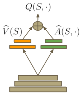
In reinforcement learning, the advantage function [9] can be defined as follows:

\[A(s, a) = Q(s, a) - V(s)\]

If \(Q(s, a)\) represents the value of a given action \(a\) chosen in state \(s\), \(V(s)\) represents the value of the state independent of action. This property leads to the definition \(V(s) = \max_aQ(s, a)\). Thus, \(A(s, a)\) provides a relative measure of the utility of actions in \(s\). The insight behind the dueling network architecture [6] is that sometimes the exact choice of action does not matter so much, and so the state could be more explicitly modelled, independent of the action. Another advantage (no pun intended) is that when bootstrapping in reinforcement learning (using estimated values to learn), it helps to have a good estimate of \(V(s)\). Therefore, the function can be built into the architecture of the network (much like with Residual Networks):

When altering the DQN code, it only requires replacing the fully connected layers at the top with the following:

-- Value approximator V^(s)
local valStream = nn.Sequential()
valStream:add(nn.Linear(convOutputSize, hiddenSize))
valStream:add(nn.ReLU(true))
valStream:add(nn.Linear(hiddenSize, 1)) -- Predicts value for state

-- Advantage approximator A^(s, a)
local advStream = nn.Sequential()
advStream:add(nn.Linear(convOutputSize, hiddenSize))
advStream:add(nn.ReLU(true))
advStream:add(nn.Linear(hiddenSize, m)) -- Predicts action-conditional advantage

-- Streams container
local streams = nn.ConcatTable()
streams:add(valStream)
streams:add(advStream)

-- Add dueling streams
net:add(streams)
-- Add dueling streams aggregator module
net:add(DuelAggregator(m))

The aggregator module is a little more involved, but can be constructed using Torch’s standard table containers.

Training

As mentioned previously, training on the ALE can take over a week to complete. One game that is good for quicker testing is Pong, as it should achieve perfect or near-perfect results in about 1/10 of the normal training iterations (typically a day on a GPU). For those who want to see more immediate results, the code is also set up to play Catch - a 24\(\times\)24px black & white environment where the agent’s paddle at the bottom has to catch a falling ball.

Results

Below we can see the difference between the original DQN, the double DQN (DDQN) [10] (which uses an improved version of the Q-learning update rule), and the dueling DQN on Space Invaders. As in the original paper, the dueling DQN also utilises the same update rule as the DDQN.

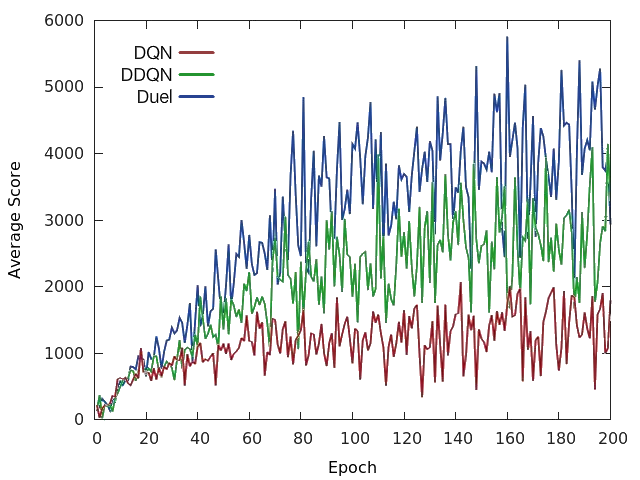
Overall, the dueling network architecture achieved better performance than the original DQN and DDQN in nearly all games [6]. More importantly, this concept may be used in tandem with other advances on the DQN, which means that it can be used as just one component of a successful deep reinforcement learning agent.

Conclusion

This post discussed how DQNs are able to learn successful policies in high-dimensional visual domains, and can be made more powerful by purely architectural additions. It also looked at how CNN visualisation techniques can be used to understand a DQN’s actions.

Acknowledgements

DeepMind for releasing their source code [1], which was used as a reference.
Laszlo Keri and other contributors to the repo.

References

1. Mnih, V., Kavukcuoglu, K., Silver, D., Rusu, A. A., Veness, J., Bellemare, M. G., … & Petersen, S. (2015). Human-level control through deep reinforcement learning. Nature, 518(7540), 529-533.
2. Bellemare, M. G., Naddaf, Y., Veness, J., & Bowling, M. (2013). The Arcade Learning Environment: An Evaluation Platform for General Agents. Journal of Artificial Intelligence Research, 47, 253-279.
3. Tesauro, G. (1994). TD-Gammon, a self-teaching backgammon program, achieves master-level play. Neural computation, 6(2), 215-219.
4. Riedmiller, M. (2005). Neural fitted Q iteration–first experiences with a data efficient neural reinforcement learning method. In Machine Learning: ECML 2005 (pp. 317-328). Springer Berlin Heidelberg.
5. Lin, L. J. (1992). Self-improving reactive agents based on reinforcement learning, planning and teaching. Machine learning, 8(3-4), 293-321.
6. Wang, Z., de Freitas, N., & Lanctot, M. (2015). Dueling Network Architectures for Deep Reinforcement Learning. arXiv preprint arXiv:1511.06581.
7. Simonyan, K., Vedaldi, A., & Zisserman, A. (2013). Deep inside convolutional networks: Visualising image classification models and saliency maps. arXiv preprint arXiv:1312.6034.
8. Springenberg, J. T., Dosovitskiy, A., Brox, T., & Riedmiller, M. (2014). Striving for simplicity: The all convolutional net. arXiv preprint arXiv:1412.6806.
9. Baird III, L. C. (1993). Advantage updating (No. WL-TR-93-1146). Wright Lab Wright-Patterson AFB OH.
10. Van Hasselt, H., Guez, A., & Silver, D. (2015). Deep reinforcement learning with double Q-learning. arXiv preprint arXiv:1509.06461.